Aperture (pyoof.aperture)
Introduction
The aperture sub-package contains related distributions/functions to the aperture distribution, \(\underline{E_\text{a}}(x, y)\). The aperture distribution is a two dimensional complex distribution, hence has an amplitude and a phase. The amplitude is represented by the blockage distribution, \(B(x, y)\), and the illumination function, \(E_\text{a}(x, y)\). The phase is given by the aperture phase distribution, \(\varphi(x, y)\) and the optical path difference (OPD) function, \(\delta(x,y;d_z)\) [Stutzman].
The collection of all distributions/functions for the aperture distribution is then,
Among them, the blockage distribution and OPD function are strictly dependent on the telescope geometry, which is the reason why they are gathered in the telgeometry sub-package.
Note
All mentioned Python functions are for a two dimensional analysis and they require as an input meshed values. They can also be used in one dimensional analysis by adding y=0 to each of the Python functions. Although their analysis in the pyoof package is strictly two-dimensional.
- To generate meshed values simply use the
meshgridroutine. >>> import numpy as np >>> from astropy import units as u >>> x = np.linspace(-50, 50, 100) * u.m >>> xx, yy = np.meshgrid(x, x) # values in a grid
Note
A Jupyter notebook tutorial for the aperture sub-package is provided in the aperture.ipynb on the GitHub repository.
Lastly there is another distribution left which is the (field) radiation pattern (voltage reception pattern), \(F(u, v)\), which is the direct Fourier Transform (in two dimensions) of the aperture distribution (both of them being complex numbers).
The (field) radiation pattern is the most extensive function in this sub-package. The standard Python package fft2 is used to compute the FFT in two dimensions.
Using aperture
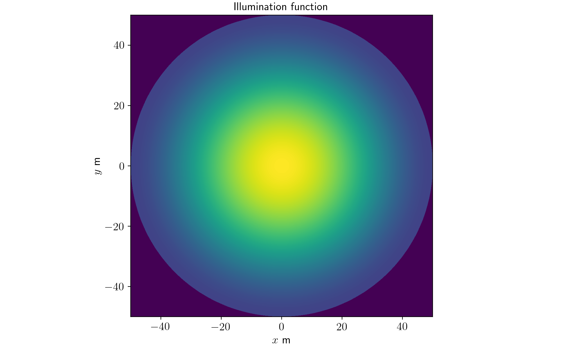
Using the aperture package is really simple, for example the illumination function, \(E_\text{a}(x, y)\),
import numpy as np
import matplotlib.pyplot as plt
from astropy import units as u
from pyoof import aperture

pr = 50 * u.m  # primary reflector radius
x = np.linspace(-pr, pr, 1000)
y = x.copy()
xx, yy = np.meshgrid(x, y)

I_coeff = [1, -14 * u.dB, 2, 0 * u.m, 0 * u.m]  # [amp, c_dB, q, x0, y0]

Ea = aperture.illum_parabolic(xx, yy, I_coeff, pr)
Ea[(xx ** 2 + yy ** 2 > pr ** 2)] = 0  # circle shape

fig, ax = plt.subplots()

ax.imshow(
    X=Ea,
    extent=[-pr.to_value(u.m), pr.to_value(u.m)] * 2,
    cmap='viridis'
    )
ax.set_xlabel('$x$ m')
ax.set_ylabel('$y$ m')
ax.set_title('Illumination function')
(Source code, png, hires.png, pdf)
The aperture only uses standard Python libraries, but what needs special consideration are the Python functions with the parameter K_coeff, coming up.
Note
The illumination function is set free to the user but in pyoof we have included two illum_parabolic with two degrees of freedom (c_dB and q in the I_coeff key) and illum_gauss with a single degree of freedom (c_dB).
For more see [LoYeun] Chapter 15: Reflector Antennas.
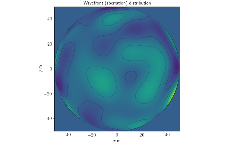
Wavefront (aberration) distribution \(W(x, y)\)
The wavefront (aberration) distribution [Welford], \(W(x, y)\), is strictly related to the aperture phase distribution (see Jupyter notebook, zernike.ipynb on GitHub), and it is the basis of the nonlinear least squares minimization done by the pyoof package.
Note
The Zernike circle polynomial coefficients, given by K_coeff are the basic structure for the aperture phase distribution. The polynomial order \(n\) is given by \((n+1)(n+2)/2\), or total number of polynomials. See zernike.
One basic example is to plot \(W(x, y)\) with a random set of Zernike circle polynomial coefficients.
import numpy as np
import matplotlib.pyplot as plt
from astropy import units as u
from pyoof import aperture, cart2pol

pr = 50 * u.m                       # primary reflector radius
n = 10                              # order polynomial
N_K_coeff = (n + 1) * (n + 2) // 2  # max polynomial number
K_coeff = np.random.normal(0., .1, N_K_coeff)

x = np.linspace(-pr, pr, 1000) # Generating the mesh
xx, yy = np.meshgrid(x, x)
r, t = cart2pol(xx, yy)
r_norm = r / pr                # polynomials under unitary circle

W = aperture.wavefront(rho=r_norm, theta=t, K_coeff=K_coeff)
W[xx ** 2 + yy ** 2 > pr ** 2] = 0

fig, ax = plt.subplots()
ax.contour(xx, yy, W, colors='k', alpha=0.3)
ax.imshow(
    X=W,
    extent=[-pr.to_value(u.m), pr.to_value(u.m)] * 2,
    origin='lower',
    cmap='viridis'
    )

ax.set_title('Wavefront (aberration) distribution')
ax.set_ylabel('$y$ m')
ax.set_xlabel('$x$ m')
(Source code, png, hires.png, pdf)

Aperture phase distribution \(\varphi(x, y)\)
The calculation of the aperture phase distribution, phase, follows the same guidelines as the wavefront (aberration) distribution, wavefront. In general, the problem will only focus on the aperture phase distribution, and not on the wavefront (aberration) distribution. To compute the phase-error simply,
import numpy as np
import matplotlib.pyplot as plt
from astropy import units as u
from pyoof import aperture

pr = 50 * u.m                       # primary reflector radius
n = 5                               # order polynomial
N_K_coeff = (n + 1) * (n + 2) // 2  # max polynomial number
K_coeff = np.random.normal(0., .1, N_K_coeff)

x, y, phi_notilt_nopiston = aperture.phase(
    K_coeff=K_coeff,
    piston=False,
    tilt=False,
    pr=pr
    )
phi = aperture.phase(
    K_coeff=K_coeff,
    piston=True,
    tilt=True,
    pr=pr
    )[2]

levels = np.linspace(-2, 2, 9)

fig, ax = plt.subplots(ncols=2, sharey=True)
fig.subplots_adjust(wspace=0.1)

for i, data in enumerate([phi_notilt_nopiston.value, phi.value]):
    ax[i].imshow(
        X=data,
        extent=[-pr.value, pr.value] * 2,
        origin='lower',
        cmap='viridis'
        )
    ax[i].contour(x, y, data, levels=levels, alpha=0.3, colors='k')
    ax[i].set_xlabel('$x$ m')

ax[0].set_ylabel('$y$ m')
ax[0].set_title('$\\varphi(x, y)$ no-tilt and no-piston')
ax[1].set_title('$\\varphi(x, y)$')
(Source code, png, hires.png, pdf)
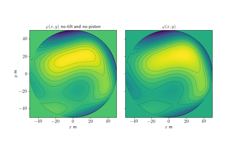
To study the aberration in the aperture phase distribution it is necessary to remove some telescope effects. These are the tilt terms that are related to the telescope’s pointing, and become irrelevant, same as the piston or overall amplitude. The tilt terms also represent the average slope in the \(x\) and \(y\) directions. In the Zernike circle polynomials coefficients, the tilt terms are \(K^1_1\) and \(K^{-1}_1\). To erase their dependence they are set to zero with the option piston = False and tilt = False.
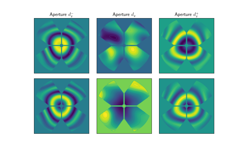
Aperture distribution \(\underline{E_\text{a}}(x, y)\)
To compute the aperture distribution, two extra functions from the telgeometry package are required. Assuming the reader knows them, it is easy to compute \(\underline{E_\text{a}}(x, y)\),
import numpy as np
import matplotlib.pyplot as plt
from astropy import units as u
from pyoof import aperture, telgeometry
pr = 50 * u.m # primary reflector radius
n = 5 # order polynomial
N_K_coeff = (n + 1) * (n + 2) // 2 # max polynomial number
K_coeff = np.random.normal(0., .1, N_K_coeff)
c = np.random.randint(-20, -8) * u.dB # First illumination degree
q = 2 # Second illumination degree
I_coeff = [1, c, q, 0 * u.m, 0 * u.m]
# Generating the mesh
x = np.linspace(-pr, pr, 1000)
xx, yy = np.meshgrid(x, x)
# For these functions see telgeometry sub-package
telgeo = [telgeometry.block_effelsberg(), telgeometry.opd_effelsberg, pr]
Ea = []
for d_z in [-2.2, 0, 2.2] * u.cm:
Ea.append(
aperture.aperture(
x=xx, y=yy,
K_coeff=K_coeff,
I_coeff=I_coeff,
d_z=d_z, # radial offset
wavel=9 * u.mm, # observation wavelength
illum_func=aperture.illum_parabolic,
telgeo=telgeo # see telgeometry sub-package
)
)
extent = [-pr.value, pr.value] * 2
fig, axes = plt.subplots(ncols=3, nrows=2)
fig.subplots_adjust(hspace=0.1, wspace=0)
ax = axes.flat
for i in range(3):
ax[i].imshow(Ea[i].real, cmap='viridis', origin='lower', extent=extent)
ax[i + 3].imshow(
Ea[i].imag, cmap='viridis', origin='lower', extent=extent
)
ax[i].contour(xx, yy, Ea[i].real, cmap='viridis')
ax[i + 3].contour(xx, yy, Ea[i].imag, cmap='viridis')
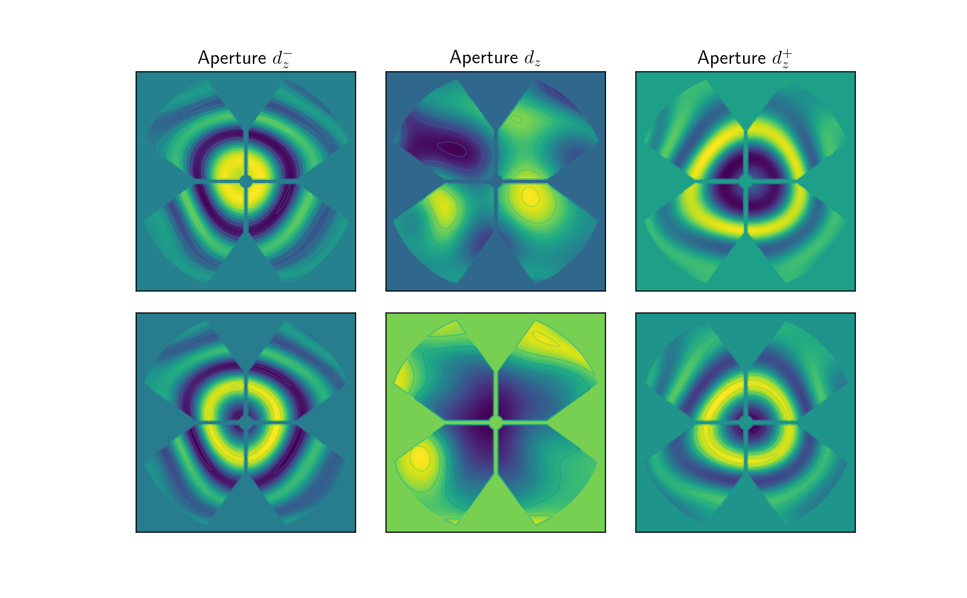
ax[0].set_title('Aperture $d_z^-$')
ax[1].set_title('Aperture $d_z$')
ax[2].set_title('Aperture $d_z^+$')
for _ax in ax:
_ax.set_xticklabels([])
_ax.set_yticklabels([])
_ax.xaxis.set_ticks_position('none')
_ax.yaxis.set_ticks_position('none')
(Source code, png, hires.png, pdf)

As mentioned before the aperture distribution is complex, and depends on the radial offset added to defocus the telescope. Depending on that its shape in real and imaginary parts will change. In general, the aperture distribution will not be used for the OOF holography study, only the power pattern and phase-error will be used for visual inspection.
In contrast the voltage reception pattern has the same inputs, except for the fft2 routine, which requires two more important parameters. These are resolution and box_factor. This is simply executed by,
import numpy as np
import matplotlib.pyplot as plt
from astropy import units as u
from pyoof import aperture, telgeometry

pr = 50 * u.m                       # primary reflector radius
n = 5                               # order polynomial
N_K_coeff = (n + 1) * (n + 2) // 2  # max polynomial number
K_coeff = np.random.normal(0., .1, N_K_coeff)

c = np.random.randint(-20, -8) * u.dB      # First illumination degree
q = 2                                      # Second illumation degree
I_coeff = [1, c, q, 0 * u.m, 0 * u.m]

telgeo = [telgeometry.block_effelsberg(), telgeometry.opd_effelsberg, pr]

F = aperture.radiation_pattern(
    K_coeff=K_coeff,
    I_coeff=I_coeff,
    d_z=0 * u.cm,
    wavel=9 * u.mm,
    illum_func=aperture.illum_parabolic,
    telgeo=telgeo,
    resolution=2 ** 8,
    box_factor=5 * pr
    )
References
- Stutzman
Stutzman, W. and Thiele, G., 1998. Antenna Theory and Design. Second edition. Wiley.
- Welford
Welford, W., 1986. Aberration of Optical Systems. The Adam Hilger Series on Optics and Optoelectronics.
- LoYeun
Lo, Yuen T., and S. W. Lee., 2013. Antenna Handbook: theory, applications, and design. Springer Science & Business Media.
See Also
Reference/API
pyoof.aperture Package
This sub-package contains all necessary functions to compute the aperture distribution and the (field) radiation pattern, and is ready to be used by the least squares minimization.
Functions
|
Aperture distribution, \(\underline{E_\mathrm{a}}(x, y)\). |
|
Computes the random-surface-error efficiency, \(\varepsilon_\mathrm{rs}\), using the Ruze’s equation. |
|
Illumination function, \(E_\mathrm{a}(x, y)\), Gaussian, sometimes called apodization, taper or window. |
|
Illumination function, \(E_\mathrm{a}(x, y)\), parabolic taper on a pedestal, sometimes called apodization, taper or window. |
|
Aperture phase distribution (or phase-error), \(\varphi(x, y)\), for an specific telescope primary reflector. |
|
Spectrum or (field) radiation pattern, \(F(u, v)\), it is the FFT2 computation of the aperture distribution, \(\underline{E_\mathrm{a}} (x, y)\), in a rectangular grid. |
|
Computes the wavefront (aberration) distribution, \(W(x, y)\). |