Zernike circle polynomials (`pyoof.zernike`)¶

Introduction¶

The Zernike circle polynomials [Virendra] were introduced by Frits Zernike (winner Nobel prize in physics 1953), for testing his phase contrast method in circular mirror figures. The polynomials were used by Ben Nijboer to study the effects of small aberrations on diffracted images with a rotationally symmetric origin on circular pupils.

The studies on the wavefront (aberration) distribution, have been classically described as a power series, where it is possible to expand it in terms of orthonormal polynomials in the unitary circle. Although, there is a wide range of polynomials that fulfill this condition, the Zernike circle polynomials have certain properties of invariance that make them unique.

Mathematical definitions¶

There are no conventions assigned on how to enumerate the Zernike circle polynomials. In the pyoof package uses the same letters and conventions from [Born]. The Zernike circle polynomials can be expressed as a multiplication of radial and angular sections. The radial section it is called radial polynomials, and its generating function is given by,

\[R^{\pm m}_n (\varrho) = \frac{1}{\left(\frac{n-m}{2}\right)!\cdot\varrho^m}\left\{\frac{\text{d}}{\text{d}\left(\varrho^2\right)} \right\}^{\frac{n-m}{2}} \left\{ \left( \varrho^2 \right)^{\frac{n+m}{2}} \cdot \left( \varrho^2 -1 \right)^{\frac{n-m}{2}} \right\}.\]

The above expression only works when \(n-m\) is even, otherwise it vanishes. Then the Zernike circle polynomials, \(U^\ell_n(\varrho, \vartheta)\), are,

\[\begin{split}U^\ell_n(\varrho, \vartheta) = R^m_n(\varrho) \cdot \cos m\vartheta \qquad \ell \geq 0, \\ U^\ell_n(\varrho, \vartheta) = R^m_n(\varrho) \cdot \sin m\vartheta \qquad \ell < 0.\end{split}\]

The angular dependence is given by \(\ell\), and \(m=\ell\), and the order of the polynomial is given by \(n\). Low orders of the Zernike circle polynomials are closely related to classical aberrations. Up to order \(n=4\) there are 15 polynomials, this is given by the formula,

\[\frac{(n+1)(n+2)}{2}.\]

The following table shows the Zernike circle polynomials up to order four.

`Order` \(n\)	`Angle` \(\ell\)	`Polynomial` \(U^\ell_n(\varrho, \vartheta)\)	`Name`
\(0\)	\(0\)	\(1\)	Piston
\(1\)	\(-1\)	\(\varrho\sin\vartheta\)	\(y\)-tilt
\(1\)	\(1\)	\(\varrho\cos\vartheta\)	\(x\)-tilt
\(2\)	\(-2\)	\(\varrho^2\sin2\vartheta\)
\(2\)	\(0\)	\(2\varrho^2-1\)	Defocus
\(2\)	\(2\)	\(\varrho^2\cos2\vartheta\)	Astigmatism
\(3\)	\(-3\)	\(\varrho^3\sin3\vartheta\)
\(3\)	\(-1\)	\((3\varrho^3-2\varrho)\sin\vartheta\)	Primary \(y\)-coma
\(3\)	\(1\)	\((3\varrho^3-2\varrho)\cos\vartheta\)	Primary \(x\)-coma
\(3\)	\(3\)	\(\varrho^3\cos3\vartheta\)
\(4\)	\(-4\)	\(\varrho^4\cos4\vartheta\)
\(4\)	\(-2\)	\((4\varrho^4-3\varrho^2)\sin2\vartheta\)
\(4\)	\(0\)	\(6\varrho^4-6\varrho^2+1\)	Primary spherical
\(4\)	\(2\)	\((4\varrho^4-3\varrho^2)\cos2\vartheta\)	Second astigmatism
\(4\)	\(4\)	\(\varrho^4\cos4\vartheta\)

The Zernike circle polynomials can be used to represent, in a convenient way, the wavefront (aberration) distribution, \(W(x, y)\), [Wyant]. It is convenient, because low orders are related to classical aberrations (from optic physics), as well as their lower orders are able to represent mid- to low-resolution aperture phase distribution maps, \(\varphi(x, y)\). The general expression concerning them is given by,

\[\varphi(x, y) = 2\pi \cdot W(x, y) = 2\pi \cdot \sum_{n, \ell} K_{n\ell}U^\ell_n(\varrho, \vartheta),\]

where \(K_{n\ell}\) are the Zernike circle polynomial coefficients. The final output from the pyoof package is to find such coefficients and then make a representation of the aberration in the (telescope) aperture plane. The wavefront (aberration) distribution, wavefront, is a function listed in the aperture sub-package. The order of the \(K_{n\ell}\) coefficients will depend on the order of the polynomials.

Warning

The order of magnitude of the Zernike circle polynomial coefficients (\(K_{n\ell}\)) will vary on what conventions are used to generate them. There are some conventions that require a normalization constant.

Using `zernike`¶

To use the polynomials from the zernike is really easy. First import the sub-package and start using the default structure:

>>> import numpy as np
>>> from astropy import units as u
>>> from pyoof import zernike  # calling the sub-package
>>> rho = np.linspace(0, 1, 10) * u.m
>>> R40 = zernike.R(n=4, m=0, rho=rho / rho.max())
>>> R40
<Quantity [ 1.        ,  0.92684042,  0.71833562,  0.40740741,  0.04892547,
           -0.28029264, -0.48148148, -0.43392775,  0.00502972,  1.        ]>

To plot the polynomials first it is required to construct a grid.

import numpy as np
import matplotlib.pyplot as plt
from astropy import units as u
from pyoof import zernike, cart2pol

radius = 1 * u.m
x = np.linspace(-radius, radius, 1000)
xx, yy = np.meshgrid(x, x)
rho, theta = cart2pol(xx, yy)
rho_norm = rho / radius  # polynomials only work in the unitary circle

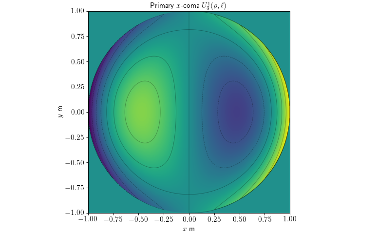
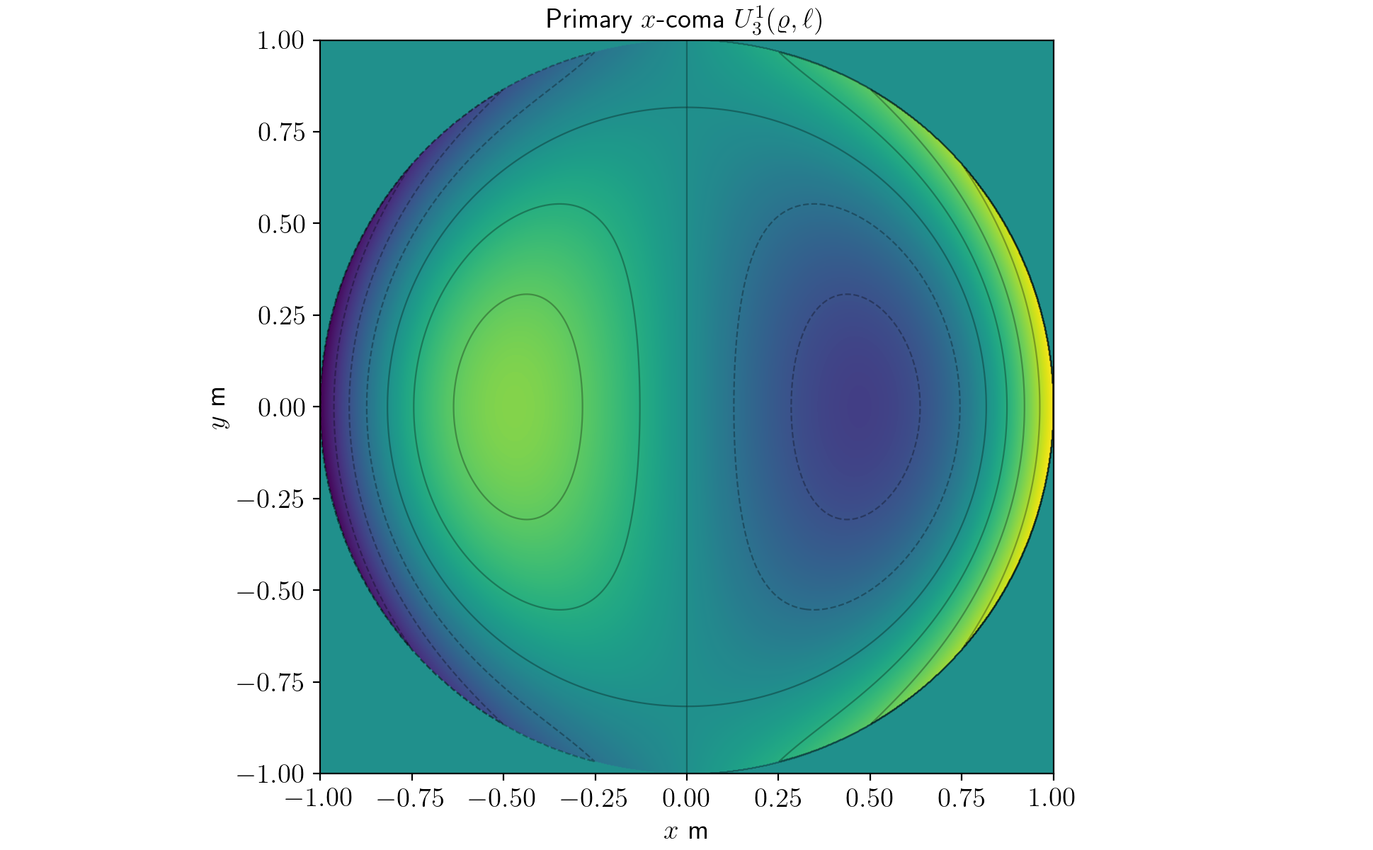
U31 = zernike.U(n=3, l=1, rho=rho_norm, theta=theta)
extent = [x.value.min(), x.value.max()] * 2

# restricting to a circle shape
U31[(xx ** 2 + yy ** 2 > radius ** 2)] = 0

fig, ax = plt.subplots()
ax.imshow(U31, extent=extent, origin='lower', cmap='viridis')
ax.contour(xx, yy, U31, alpha=0.3, colors='k')
ax.set_title('Primary $x$-coma $U^1_3(\\varrho, \\ell)$')
ax.set_xlabel('$x$ m')
ax.set_ylabel('$y$ m')

(Source code, png, hires.png, pdf)

Note

At the time of using the function U make sure that the radius is normalized by its maximum. The Zernike circle polynomials are only orthonormal under the unitary circle.

For a more in-depth example of their usage go to the Jupyter notebook zernike.ipynb.

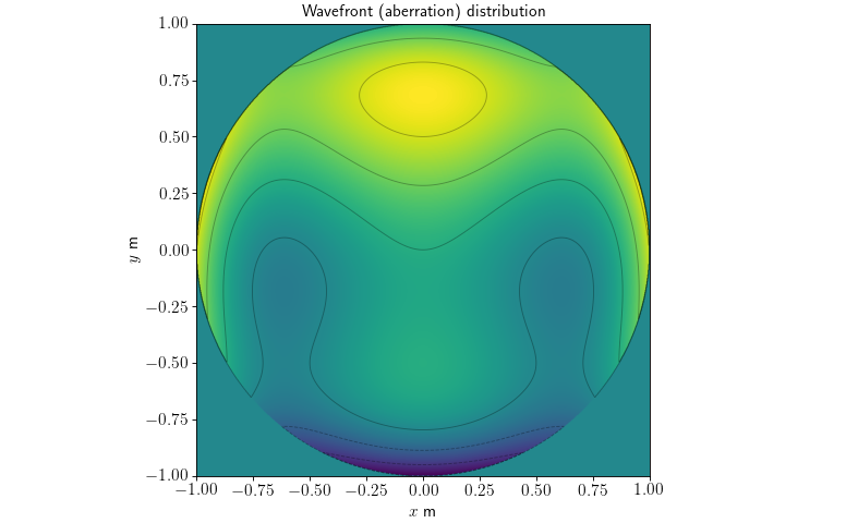
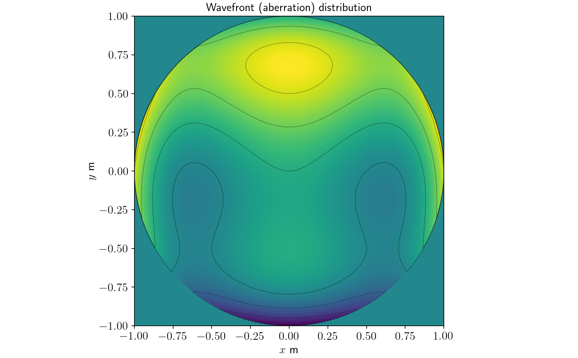
An example of wavefront (aberration) distribution could be the following,

\[W(x, y) = U^0_0 + \frac{1}{10}\cdot U^{-1}_1 + \frac{1}{5} \cdot U^{2}_4\]

Then a plot of such function will be,

import numpy as np
import matplotlib.pyplot as plt
from astropy import units as u
from pyoof import zernike, cart2pol

radius = 1 * u.m
x = np.linspace(-radius, radius, 1000)
xx, yy = np.meshgrid(x, x)
rho, theta = cart2pol(xx, yy)
rho_norm = rho / radius  # polynomials only work in the unitary circle

K_coeff = [1/10, 1 / 5, 1/ 5]
_U = [
    zernike.U(n=0, l=0, rho=rho_norm, theta=theta),
    zernike.U(n=1, l=-1, rho=rho_norm, theta=theta),
    zernike.U(n=4, l=2, rho=rho_norm, theta=theta)
    ]

W = sum(K_coeff[i] * _U[i] for i in range(3))  # wavefront distribution
extent = [x.value.min(), x.value.max()] * 2

# restricting to a circle shape
W[(xx ** 2 + yy ** 2 > radius ** 2)] = 0

fig, ax = plt.subplots()
ax.imshow(W, extent=extent, origin='lower', cmap='viridis')
ax.contour(xx, yy, W, alpha=0.3, colors='k')
ax.set_title('Wavefront (aberration) distribution')
ax.set_xlabel('$x$ m')
ax.set_ylabel('$y$ m')

(Source code, png, hires.png, pdf)

References¶

Born: Born, M. and Wolf, E., 1959. Principles of Optics: Electromagnetic Theory of Propagation, Interference and Diffraction of Light. Pergamon Press.
Virendra: Virendra N. Mahajan, “Zernike Circle Polynomials and Optical Aberrations of Systems with Circular Pupils”, Appl. Opt. 33, 8121-8124 (1994)
Wyant: Wyant, James C., and Katherine Creath. “Basic Wavefront Aberration Theory for Optical Metrology.” (1992).

Reference/API¶

pyoof.zernike Package¶

This package contains analyic functions useful for Zernike polynomials and the aperture distribution function.

Functions¶

`R`(n, m, rho)	Radial Zernike polynomials generator (\(R^m_n(\varrho)\) from Born & Wolf definition).
`U`(n, l, rho, theta)	Zernike circle polynomials generator (\(U^\ell_n(\varrho, \varphi)\) from Born & Wolf definition).

Navigation

Zernike circle polynomials (pyoof.zernike)¶